Category Archives: Energy Trading

Natural gas winter volatility p-value simulation

Natural gas prices are more volatile during the winter heating season. I’ve adapted the code from Data Analysis for the Life Sciences to use natural gas daily price change and simulate a p-value.

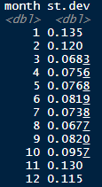
Actual monthly natural gas volatility since 2010:

ng1 %>% group_by(month) %>% summarize(st.dev = sd(ng.diff)) #find the st. dev. of each month’s prices

Separate daily natural gas prices into winter and not winter:

ng.not.winter <- ng1 %>% dplyr::filter(!month %in% c(“1”, “2”)) #control group
ng.winter <- ng1 %>% dplyr::filter(month %in% c(“1”, “2”)) #treatment group

Find the real difference in price volatility (standard deviation of price):

month.diff <- sd(ng.winter$ng1) – sd(ng.not.winter$ng1)

Create a null distribution by sampling:

set.seed(1)
n <- 10000
samp.size <- 12
null <- vector(“numeric”, n) #create a vector for the null distribution, holding the differences between means of samples from the same population

for(i in 1:n) {
ng.not.winter.sample <- sample(ng.not.winter$ng1, samp.size) #sampling from population of control
ng.winter.sample <- sample(ng.not.winter$ng1, samp.size) #sampling from population of control
null[i] <- sd(ng.winter.sample) – sd(ng.not.winter.sample)
}

mean(null >= month.diff) #p-value

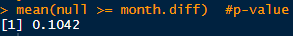
Not below 5%, but not bad. The p-value would decrease if we increased the sample size.

10% of samples from the control group (non-winter) have differences greater than the true difference. This is the p-value.

hist(null, freq=TRUE)
abline(v=month.diff, col=”red”, lwd=2)

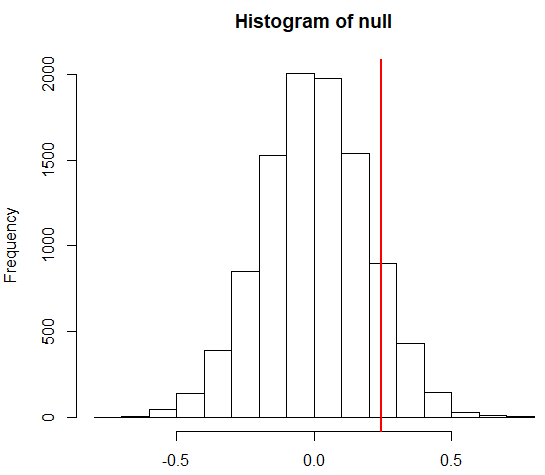
The histogram looks normal, so using a normal approximation should give a similar answer:

1 – pnorm(month.diff, mean(null), sd(null))

Return calculations in R

Discrete returns the long way. This assumes the prices are in an xts object. stats::lag is specified since dplyr can mask the stats lag function with its own lag function:

head(diff(prices.xts)[2:n-1]/stats::lag(prices.xts, 1))

The easy way, with the PerformanceAnalytics package:

library(PerformanceAnalytics)
head(Return.calculate(prices.xts, method = “discrete”))

Check they’re the same:

Log returns the long way, this time removing NAs:

na.omit(diff(log(prices.xts))

With PerformanceAnalytics:

prices.ret <-na.omit((Return.calculate(prices.xts, method = “log”)))

Convert to a data.frame, rename date column, remove NAs if any:

data.frame(index(prices.ret), coredata(prices.ret)) %>% dplyr::rename(date = index.prices.ret.) %>% na.omit()

The message of the forward curve

From Reuters today:

“In late 2014 and again in late 2015, traders and refiners raced to buy as much crude as possible and put it into storage to profit from a big contango structure in the futures market.

But the strategy depends on the contango remaining wide enough to cover all the costs of financing and storing the physical crude.

As the contango in Brent narrows sharply, strategies which depend on selling Brent futures are becoming unprofitable (Hedge funds bet on tightening oil market despite Doha debacle, Reuters, April 19).

To the extent traders and refiners are financing and storing extra stock with Brent futures, the barrels are likely to be sold if the market remains in a narrow contango or moves deeper into backwardation.”

Oil Rigs, Production, Imports, and Storage

US oil rigs in operation have fallen from a high of 1609 in October 2014 to 372 last week, according to Baker Hughes.  US oil production has fallen from 9.61 million barrels/day in June 2015 to 9.02 mbd last week, according to the EIA.

However, imports of oil into the US has increased during that same time, and the total amount of oil in storage in the US has risen.

oil rigs, prod, impoil storage


Condensate Splitters and the WTI-Brent Spread

http://www.reuters.com/article/us-usa-oil-splitters-analysis-idUSKBN0UB08Z20151228

New splitter projects look less attractive as WTI-Brent tightens.  This tightening has more to do with the reduced light oil production in the U.S. and less to do with removing the oil export ban.  A future oil price rise will incentivize more U.S. shale production, widening the WTI-Brent spread out again, which would make splitters more attractive.

wtibrent

Multiple Lines in One ggplot Graph in R

> library(reshape2)
> library(ggplot2)
> date = data$date
> price1 = data$wti
> price2 = data$ulsd
> df = data.frame(date,price1,price2)
> df2 = melt(data = df,id.vars = "date")
> ggplot(data = df2,aes(x = date,y = value,color = variable)) + geom_line()

ggplot multiple lines

Add ylab and xlab for labels:

> a = ggplot(data = df2,aes(x = date,y = value,color = variable)) + geom_line()
> a + ylab("price")


How to Create a Correlation of Multiple Time Series in R

With a matrix of data like this (you should calculate correlations on returns, but absolute prices are used here for the example):

excelpic

Name your desired column vectors:

> wti = data$wti
> brent = data$brent
> lls = data$lls
> mars = data$mars


> dataframe = data.frame(wti,brent,lls,mars)
> COR = cor(dataframe)
> head(round(COR,2))
       wti brent  lls mars
wti   1.00  0.97 0.96 0.96
brent 0.97  1.00 0.99 0.99
lls   0.96  0.99 1.00 1.00
mars  0.96  0.99 1.00 1.00


If the correlation matrix comes back with “NA”s, use the na.omit command:

> clean = na.omit(dfrm)
> cor(clean)


Load “corrplot” package:

> library(corrplot)


> corrplot(COR,method = "number")


corrplot

See here for more on corrplot:

https://cran.r-project.org/web/packages/corrplot/vignettes/corrplot-intro.html

The R Cookbook has good information.

How to Subset a Vector by Another Vector in R

You have a matrix like this:

excelpic

You want to only look at Q1 prices for the spread between two products.  You can subset the price vectors by the qtr vector like this:

gcq116 = data[data$qtr==1,c("gc87q116")]
rbobq116 = data[data$qtr==1,c("rbobq116")]


Create the date vector:

> dateqtr1 = data[data$qtr==1,c("date")]


You now have two price vectors showing only the Q1 prices.  Graph the spread between the two vectors like this:

> qplot(dateqtr1,gcq116 - rbobq116)


which returns this:

subset prices