Category Archives: Financial Mathematics

Standard error of a difference of sample means

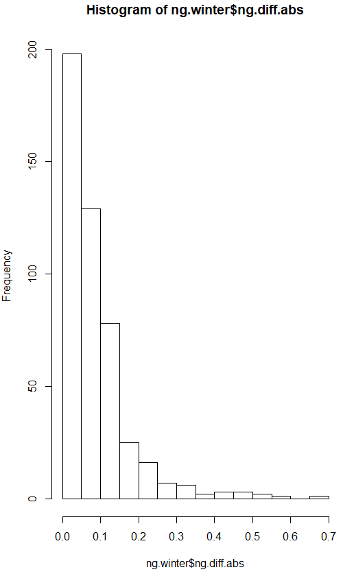
The variance of the difference of two random variables is the sum of the two variances. We sample 30 observations (usually large enough according to the CLT) from winter and not winter absolute daily price changes. The absolute daily changes appear log normal, but according to the Central Limit Theorem the distribution of the samples will be normal, assuming the sample size is large enough:

Now calculate the standard error of the difference of the sample means (or the sum of the sample means):

Calculate the difference in sample means and then calculate the t-statistic. Dividing a random variable (diff) by its own standard error gives a new random variable with a standard error of 1:

Tstat should be approximately normal with mean 0 and se 1. Assuming that tstat is normal, how often would a normally distributed random variable exceed tstat? The p-value is .107, not statistically significant at the common .05 level:

Central Limit Theorem simulation

Again, reworking examples from the great Data Analysis for the Life Sciences using commodities data. This example is interesting because the authors show how to use sapply, while before they used for loops. One of the great benefits of this book is the use of more advanced functional programming and iteration techniques, both of which are used in this example.

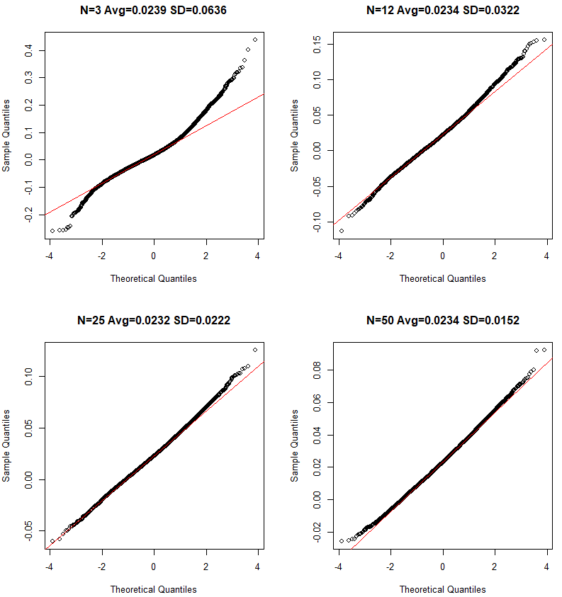
Here we are taking different sample sizes from the absolute values of the daily changes of winter natural gas and !winter natural gas and comparing the differences. We know that the 2010-today difference in the means is 0.0233, and that the standard deviation of the sample distribution should decrease as sample size increases.

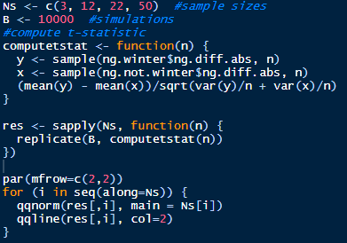
This code uses sapply to apply each of the four Ns to the user-created function inside sapply. It then uses a for loop to create charts for the results from each of the four sample sizes, adding the sample average and standard deviation in each title.

Central Limit Theorem

Definition: when the sample size is large enough, the average of a random sample from a population follows a normal distribution centered at the population average, with a sample standard deviation (standard error) equal to the population standard deviation divided by the square root of the sample size.

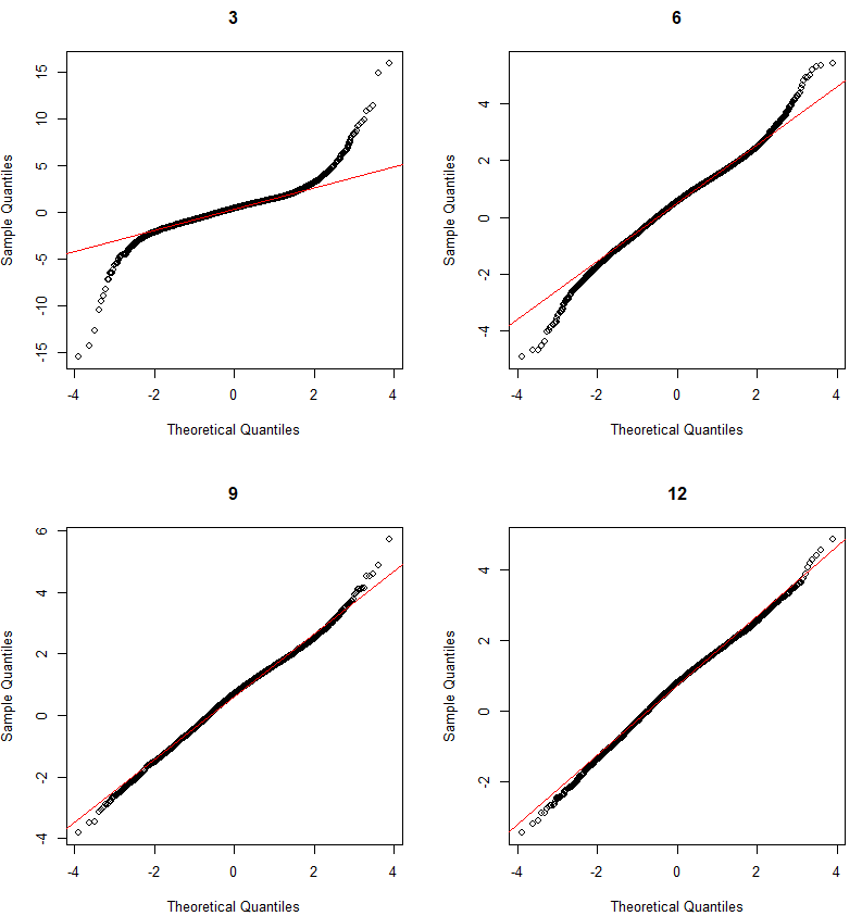
The average of this ratio is approximated by a standard normal distribution:

In the natural gas example, we have two populations (winter and not winter), and we can define the null distribution as stating that the average daily price change of the two populations is the same. The null implies that the difference between the two average daily price changes is approximated by a normal distribution centered at zero and with a standard deviation equal to the square root of the two population variances divided by the square root of the sample size. This ratio is approximately N(0, 1):

This allows us to compute the percentage of price changes that should be within or outside certain standard deviations.

If we compare the results from sampling from the populations and taking the sample means and calculating a p-value using the normal approximation, the results are very similar:

The ratio above assumes we know the population standard deviations, but we usually don’t. The sample standard deviations are defined as:

This means that the ratio above is now (if the two sample sizes are the same):

The Central Limit Theorem says that when N is large enough this ratio is also approximated by a standard normal distribution, N(0, 1).

Population vs. Sample variance

Continuing with the natural gas data, we define our population as all Henry Hub daily prices since Jan 1, 2010. The formula for population variance is

When using the “var” R function to calculate population variance we have to correct by multiplying by (n-1)/n. This is because the “var” function calculates sample variance.

The standard deviation is just the square root of the variance.

Natural gas winter volatility p-value simulation

Natural gas prices are more volatile during the winter heating season. I’ve adapted the code from Data Analysis for the Life Sciences to use natural gas daily price change and simulate a p-value.

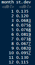
Actual monthly natural gas volatility since 2010:

ng1 %>% group_by(month) %>% summarize(st.dev = sd(ng.diff)) #find the st. dev. of each month’s prices

Separate daily natural gas prices into winter and not winter:

ng.not.winter <- ng1 %>% dplyr::filter(!month %in% c(“1”, “2”)) #control group
ng.winter <- ng1 %>% dplyr::filter(month %in% c(“1”, “2”)) #treatment group

Find the real difference in price volatility (standard deviation of price):

month.diff <- sd(ng.winter$ng1) – sd(ng.not.winter$ng1)

Create a null distribution by sampling:

set.seed(1)
n <- 10000
samp.size <- 12
null <- vector(“numeric”, n) #create a vector for the null distribution, holding the differences between means of samples from the same population

for(i in 1:n) {
ng.not.winter.sample <- sample(ng.not.winter$ng1, samp.size) #sampling from population of control
ng.winter.sample <- sample(ng.not.winter$ng1, samp.size) #sampling from population of control
null[i] <- sd(ng.winter.sample) – sd(ng.not.winter.sample)
}

mean(null >= month.diff) #p-value

Not below 5%, but not bad. The p-value would decrease if we increased the sample size.

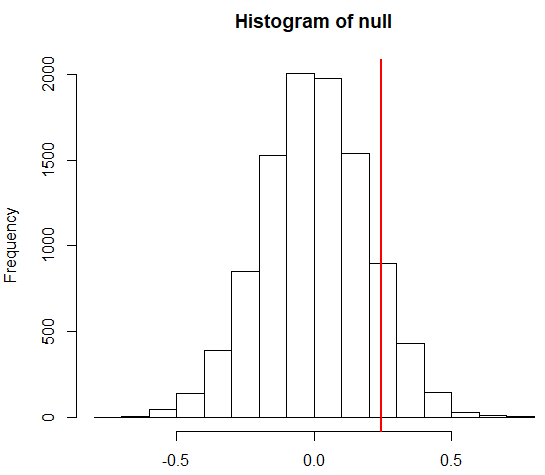
10% of samples from the control group (non-winter) have differences greater than the true difference. This is the p-value.

hist(null, freq=TRUE)
abline(v=month.diff, col=”red”, lwd=2)

The histogram looks normal, so using a normal approximation should give a similar answer:

1 – pnorm(month.diff, mean(null), sd(null))

Return calculations in R

Discrete returns the long way. This assumes the prices are in an xts object. stats::lag is specified since dplyr can mask the stats lag function with its own lag function:

head(diff(prices.xts)[2:n-1]/stats::lag(prices.xts, 1))

The easy way, with the PerformanceAnalytics package:

library(PerformanceAnalytics)
head(Return.calculate(prices.xts, method = “discrete”))

Check they’re the same:

Log returns the long way, this time removing NAs:

na.omit(diff(log(prices.xts))

With PerformanceAnalytics:

prices.ret <-na.omit((Return.calculate(prices.xts, method = “log”)))

Convert to a data.frame, rename date column, remove NAs if any:

data.frame(index(prices.ret), coredata(prices.ret)) %>% dplyr::rename(date = index.prices.ret.) %>% na.omit()

Potential Future Exposure for a Derivatives Position

Potential Future Exposure (PFE) is a simple way to measure the riskiness of a derivatives portfolio, given some statistical assumptions about the distribution of future prices of the derivative portfolio’s underlying assets.  These assumptions are wrong, but not so wrong that the PFE will not provide some valuable information. The PFE uses the model of the underlying asset price process that the Black-Scholes option formula uses, and therefore shares the same assumptions, so the PFE can illustrate some of its limitations.

The PFE is easy to model in Excel.  We start with the asset price process,

ST = Ste(r – 1/2σ^2)(T-t) +/- σZ(T-t)^2

which is described here and here. For this example I have taken the WTI Crude Oil Cal13 prices as the underlying, meaning we have a portfolio of derivatives: futures, forwards, options, or a mixture of all of them with WTI as the underlying.

The r for each month will be the LIBOR rate of corresponding term, the sigma will be the implied volatility taken from the option on each contract month, and the Z will be a confidence level that we set.  Here we use 95%, or 1.65 (standard deviations).  In Excel, use NORMSINV(.95) to get 1.65.  If our assumptions were correct, which they aren’t, 95% of the time the portfolio’s worst loss would be inside the interval we create.

Apply the above formula to each contract month, adding the second term (with the Z factor) to get the upper interval and subtracting to get the lower, and using each month’s specific r, sigma, and time to expiration for each monthly contract (T-t), and we get this result:

It is a simple matter to get an exposure in dollar terms.  We take the portfolio’s exposure in barrels, net the longs and shorts for each month, and multiply each month’s underlying by each month’s corresponding price on the lower curve (since we would be losing if the underlying went down).  If the portfolio has options, treat them as being delta barrels long or short.  This works since the option delta is calculated using the same r, sigma, S, and (T-t) as our underlying process uses here.

Note that the upper bound is farther away from the current forward curve than the lower bound.  This is due to the lognormal distribution of asset prices.  The downside is floored at zero and the upside is infinite.

N(d1) and N(d2) in the Black-Scholes Formula

N(d2) is the probability of exercise of an option with a lognormally distributed underlying following the standard BSM assumptions (drift is (r – .5σ2)(T-t)).  N(d2) defines the area of integration to give the probability of exercise and is

                Z > [ln(K/S) – (r – .5σ2)(T-t)]/σ*sqrt(T-t) = z0
meaning that the area of integration is z0 to ∞, or -∞ to  –z0, the part of the normal distribution where exercise takes place.  The option price formula can be viewed as a conditional expectation multiplied by a probability,
                e-r(T-t)[E[ST|ST > K]*N(d2) – K*N(d2)]
The conditional expectation E[ST|ST > K] can also be written as
                Se(r-.5σ^2)(T-t) + σ*sqrt(T-t)*Z
where the Z in the last term ensures that only values of the underlying S where exercise takes place are considered.  The greater the volatility σ, the greater the possible up move, the greater the area of integration, and hence the greater the conditional expectation of S.
The option price formula can now be written as
                e-r(T-t)[(Se(r-.5σ^2)(T-t) + σ*sqrt(T-t)*Z)*N(d2) – K*N(d2)]
The e(r-.5σ^2)(T-t) + σ*sqrt(T-t)*Z term can be combined with N(d2) since it is also a standard normal probability.  N(d1) is then just N(d2) +  σ*sqrt(T-t), which gives N(d1) a greater expectation based on σ.  The option price formula can now be written as
                e-r(T-t)[(Ser*N(d1) – K*N(d2)] or
                S*N(d1)- e-r(T-t)K*N(d2)
N(d1) simply takes into account the higher conditional expectation of the random underlying S versus the static K.

The Black-Scholes Differential Equation

dS = μSdt + σSdW is an Ito process with drift µ and diffusion W. The instantaneous change in W, dW, is a Brownian motion scaled by a constant σ. The increments of dW are normally distributed with mean 0 and standard deviation 1.

In Ito calculus, dt and dW behave like this when multiplied:
dWdW = dt
dtdW = 0
dtdt = 0

This means that
(dS)² = σ²S²dt.

If C is an option and S is its underlying asset then, applying Ito’s lemma and collecting terms, we get:

dC = (∂C/∂t)dt + (∂C/∂S)dS + ½(∂²C/∂S²)(dS)²

dC = (∂C/∂t)dt + (∂C/∂S)( μSdt + σSdW)
+ ½(∂²C/∂S²)σ²S²dt

dC = (∂C/∂t)dt + (∂C/∂S) μSdt + (∂C/∂S)σSdW
+ ½(∂²C/∂S²)σ²S²dt

dC = [(∂C/∂t) + μS(∂C/∂S) + ½(∂²C/∂S²) σ²S²]dt
+ (∂C/∂S)σSdW,

which is the change in the option’s value over small increments of time.

The first term, called an infinitesimal operator, has a standard, Newtonian derivative,dt, and the dW term has a stochastic, or random, derivative. To create a riskless position, the random term must be hedged away.

A position of one option and Δ shares of S is created, since all changes in the option’s value depend on changes in S. The portfolio is

Π = C + ΔS

The change in the portfolio’s value is

dΠ = dC + ΔdS.

Substituting dC and dS from above gives:

dΠ = [(∂C/∂t) + μS(∂C/∂S) + ½(∂²C/∂S²) σ²S²]dt + (∂C/∂S) σSdW + Δ[μSdt + σSdW]

and

dΠ = [(∂C/∂t) + μS(∂C/∂S) + ½(∂²C/∂S²) σ²S²]dt
+ (∂C/∂S) σSdW + ΔμSdt + ΔσSdW

Set

(∂C/∂S) σSdW + ΔσSdW = 0
to get rid of the random terms. This means that (∂C/∂S) = -Δ, and the risky terms cancel each other out, leaving

dΠ = [(∂C/∂t) + ½(∂²C/∂S²) σ²S²]dt
as the portfolio’s change in value under small changes in time. The portfolio is riskless now, so it has an expected growth of r, meaning

dΠ = rΠdt = r(C + ΔS)dt = r[C – (∂C/∂S)S]dt
Setting

r[C – (∂C/∂S)S]dt = [(∂C/∂t) + ½(∂²C/∂S²) σ²S²]dt
and cancelling terms gives

rC = (∂C/∂t) + r(∂C/∂S)S + ½(∂²C/∂S²) σ²S²
which is the Black-Scholes-Merton differential equation, a 2nd order parabolic partial differential equation. Notice that μ, the drift of the underlying S, is not in the equation. The only drift term is the risk free interest rate r.

Replacing each partial differential with its corresponding Greek letter gives

rC = Θ + rSΔ + ½ σ²S² Γ

where
∂C/∂t = Θ
∂C/∂S = Δ
∂²C/∂S² = Γ