Definition: when the sample size is large enough, the average of a random sample from a population follows a normal distribution centered at the population average, with a sample standard deviation (standard error) equal to the population standard deviation divided by the square root of the sample size.

The average of this ratio is approximated by a standard normal distribution:

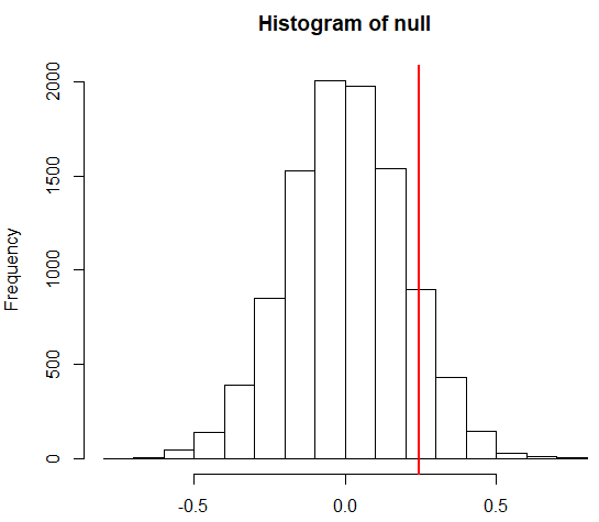
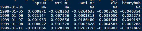
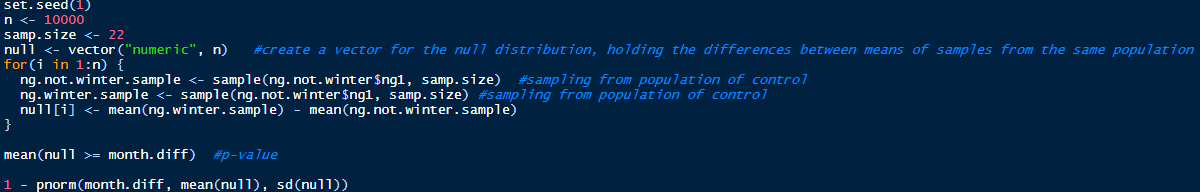
In the natural gas example, we have two populations (winter and not winter), and we can define the null distribution as stating that the average daily price change of the two populations is the same. The null implies that the difference between the two average daily price changes is approximated by a normal distribution centered at zero and with a standard deviation equal to the square root of the two population variances divided by the square root of the sample size. This ratio is approximately N(0, 1):

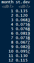
This allows us to compute the percentage of price changes that should be within or outside certain standard deviations.

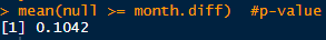
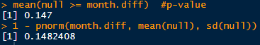
If we compare the results from sampling from the populations and taking the sample means and calculating a p-value using the normal approximation, the results are very similar:

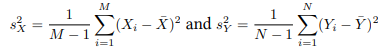
The ratio above assumes we know the population standard deviations, but we usually don’t. The sample standard deviations are defined as:

This means that the ratio above is now (if the two sample sizes are the same):

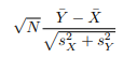
The Central Limit Theorem says that when N is large enough this ratio is also approximated by a standard normal distribution, N(0, 1).

Continuing with the natural gas data, we define our population as all Henry Hub daily prices since Jan 1, 2010. The formula for population variance is

When using the “var” R function to calculate population variance we have to correct by multiplying by (n-1)/n. This is because the “var” function calculates sample variance.

The standard deviation is just the square root of the variance.